Category: Blog

Photoshop Blend Modes – Part 2

I already introduced the blend modes Multiplication, Linear Dodge, Linear Burn and Linear Light in the first part of the series. In this article I’ll add some more that might be interesting for photographers. For one particular blend mode there is a separate third part, beause it is rather complicated and frequently used: Soft Light.

Throughout the first parts of this series, I’ll deal with the math behind the blend modes only. I plan to use these as a reference in later articles treating more practical aspects and use cases. The retouching method that triggered my research has already been given its own article: Frequency Separation.

Notation

Let me introduce a notation for inversion in addition to the ones I already introduced in the first part. Let the inverted image for an image $A$ be $\overline{A}$ . Inversion doesn’t mean anything else but subtraction of the brightness values of each pixel from 1. Thus:

$\overline{a(x,y)} = 1 - a(x,y)$ .

Or short:

$\overline{a} = 1 - a$ .

And now to the blend modes.

Color Burn

I am aware that it is slighly strange to explain something called Color Burn with black and white images. But as I said before, the math is what I will focus on first. The formulas are the same regardless or the number of channels. The formula for Color Burn is:

$f(a,b) = \left\{ \begin{array}{lr}\overline{(\frac{\overline{a}}{b})} = 1 - \frac{1- a}{b} & \text{for } b > 0\\0 & \text{for } b =0 \end{array} \right.$

Color Burn

You will notice that the whole bottom-left half drowns in black.

Color Dodge

The counterpart to Color Burn.

$f(a,b) = \left\{ \begin{array}{lr}\frac{a}{\overline{b}} = \frac{a}{1-b} & \text{for } b < 1\\1 & \text{for } b =1 \end{array} \right.$

Color Dodge

Here you get white for $a > 1-b$ .

Screen

Another rather simple but nice one:

$f(a,b) = \overline{\overline{a}\overline{b}} = 1 - (1-a)(1-b)$

Overlay and Hard Light

Overlay and Hard Light are siblings. The formulas are for Overlay:

$f(a,b) = \left\{ \begin{array}{lr} 2ab & \text{for } a < 1/2\\\overline{2\overline{a}\overline{b}} = 1 - 2(1-a)(1-b) & \text{for } a \geq 1/2 \end{array} \right.$

and for Hard Light:

$f(a,b) = \left\{ \begin{array}{lr} 2ab & \text{for } b < 1/2\\\overline{2\overline{a}\overline{b}} = 1 - 2(1-a)(1-b) & \text{for } b \geq 1/2 \end{array} \right.$

Both are combinations of slightly modified Multiply and Negative Multiply.

Overlay

Hard Light

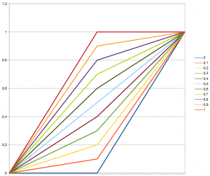
You may see it in the images, this is not a very smooth function. Plotting the brightness over a for different fixed b one gets the following:

Obviously not smooth. Make of it what you like.

50 % grey is neutral for both Overlay and Hard Light.

Vivid Light

Vivid Light can be seen as a combination of Linear Burn and Linear Dodge.

$f(a,b) = \left\{ \begin{array}{lr}\frac{a}{2(1-b)} & \text{for } b > {1/2}\\1- \frac{1-a}{2b} & \text{for } b \leq {1/2}\end{array} \right.$

Vivid Light

Other parts of this mini-series

Blend Modes – Part 1: Multiply, Linear Burn, Linear Dodge and Linear Light

Blend Modes – Part 3: Soft Light

19. January 2015
Frequency Separation
Recently I found an interesting article on frequency separation on the Fstoppers’ pages that made me curious about this method. Seems to be pretty much standard now for beauty retouching. I learned something, but the article left me with unsanswered questions:
1. Why is Linear Light the correct blend mode for rejoining the two layers created during frequency separation?
2. What exactly is the difference between addition and subtraction blend mode?
3. Why should there be a difference in the process depending on the colour-depth (8-bit versus 16-bit)?
So I decided to have a closer look. But first, I had to understand Blend Modes in general. Might be worth starting there if you have never dealt with the subject before.

The Task

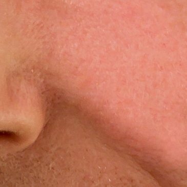
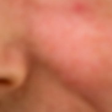
We want to split one image into two such that one of the resulting images only contains fine detail, the other the large scale changes in colour and brightness. Take the following crop from a portrait as an example:

You can see pores, a light stubble, skin texture, and you can discern features like part of a nose, a line, shadows. Here the skin texture should end up in the first image, colours and larger shadows defining the shape in the second. Later on I’d like to combine the two images again in a way that we – unless we manipulated one of the images – get the original back.

“Why?”, you may ask. Simply because after this so called frequency separation you can retouch skin-tones without having to worry about the texture and vice versa. If I wanted to get rid of the red spot you can see top right, I’d just correct the colour and brightness and leave the texture alone. All the unmodified areas will, once blended again, look unchanged. The manipulated area will look very natural. So that’s why, I’ll show you how.

But before we start, some (very little) theory.

Frequencies

Fine structures mean spatially rapid changes of brightness, or a strong local contrast. You can interpret the changes of brightness as a superposition of waves. Waves, you may remember from your physics lessons, have a frequency, in this case a spatial frequency. Fine structure means high frequency, changes over a larger distance means low frequency.

Frequency Filtering

If you are an audiophile, you may have heard of high-pass or low-pass filters used in audio equipment. They do what their names say, the low-pass lets the low frequencies pass, i.e. the bass notes, while the high-pass does the same for high frequencies. For the latter, we indeed have a ready-made filter in Photoshop. It lets the high frequencies of an image pass and blocks the low frequencies yielding an image wich is mostly grey, close to 50 %, with little deviations on a small scale. You can control the scale – or as the audiophile might say, the cutoff frequency – with the radius parameter.

Photoshop also knows low-pass filters, only they are called differently. You may be able to identify them yourself. What evens out all the small scale changes? Blurring does. There are several blur filters available. For our purpose it does not really matter which one we choose, though you have to be careful with filters like surface blur or smart blur, as they tend to create sharp edges, which mean high frequency again. I personally would use the good old workhorse gaussian blur with a rather large radius.

Back to the Task – Splitting the Image

First we have an Image A. We create two copies and modify one so we get a new image B that is different from the original A. In this example I used a gaussian blur with a radius of 6 pixels:

You see, all the fine structure is gone, no skin texture to speak of left.

Now I want to create another image C from the second copy that contains only the differences between original A and B. Should be easy, just take the second copy and use the Apply Image command of Photoshop with the blend mode Subtract with A as target and B as source and be happy. Unfortunately there is a catch.

Photoshop only allows values between 0 and 1 as result, everything below 0 and above 1 gets cut off. Not a very good idea when subtracting two very similar images, there will almost certainly be some pixels with values below 0. So what we actually do is:
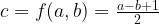
1. divide by 2
2. add ½
Thus the complete information is kept. The following formula is for a pixel-value of C:

$c = f(a,b) = \frac{a-b+1}{2}$ .

It is easy to see that nothingis lost when you look at the extremes, i.e. combinations of $a,b \in \{0,1\}$ .

Btw, I am showing all this for one channel only, for an RGB image this can be done for each channel separately.

The result of the “subtraction” is quite similar to that of Photoshop’s own High Pass filter – not exactly surprising.

Note

Photoshop can handle images with a depth of 8-bit, 16-bit or even 32-bit per pixel. The 1 I talked about above correspondes to 255, 65536 or 4294967295 respectively. The apply image dialogue offers two paramerters for the blend mode subtraction, scale and offset. For our intention we need 2 for scale – that is for the aforementioned division by two, and 128 for offset. Bit hard to recognise the addition of ½, but that is what it is. Regardless of the bit depth the offset has to be specified in parts of 256, and 128 divided by 256 happens to be ½. This is confusing, and probably the reason for some more complicated workflows I have seen.

One mentioned frequently is this (for 16-bit images):
1. invert image B
2. add the result to A
3. set the scale-parameter to 2 (i. e. divide by 2)
Looking at the math I wasn’t able to find any difference to my method. My practical tests didn’t show any either, neither for 8-bit nor for 16-bit images. If you know that inversion just means subtracting the pixel value from 1, the formula is easy:

$\frac{a+(1-b)}{2} = \frac{a-b+1}{2} = \frac{a-b}{2}+{1/2}$ .

So the answer to question three is: there is no difference.

Reassembly

Now we just need another blend mode that can reassemble the two images B and C so that, if both are unchanged, we get A again. Simply adding the pixel-values won’t work of course, we scaled and shifted the result of the subtraction. So we need to find the reverse operation. So we subtract ½ from C, multiply the result by 2 and add B.

$f(b,c) = 2(c-1/2) + b = 2c - 1 +b = b + 2c -1$ .

Surprisingly this is exactly the formula for the Linear Light blend mode. So my first question is answered as well: Linear Light is the reverse of Subtraction.

Using the Frequency Separation Technique

In practice you will of course not use Apply Image to join the hard-won separate images immediately again. You will instead use both images as layers, C over B, and set the blend mode for C to Linear Light. So you keep two layers you can work on separately. Of course you can add layers between the two, for example for non-destructive retouching. In the example I was able to remove the red spot while keeping the texture. Retouching is not within the scope of this article.

The remaining answer to question two you will find in my little series on Blend Modes – with more math and simulations.

I hope you liked my little excursus on frequency separation. If you have questions or find mistakes, do not hesitate to leave a comment.
31. December 2014
Photoshop Blend Modes – Part 1
I tried to figure out the frequency separation method for retouching portraits. Initially I didn’t really understand why which step was used. So I first had to dig deeper into the Photoshop (PS) blend modes. There’s a lot you can find on the internet regarding blend modes. Not everything I found was correct, let alone understandable for me. Especially photographers and PS users approach the subject rather intuitively, not many try to understand the math behind the tools they apply. Though that would help predicting the effects that can be achieved.

So I decided to find out what exactly happens with the goal to write a concise, but not too complicated explanation myself. The first surprise during my research was that not everybody (not even the graphic software vendors) mean the same when they talk about soft light for example. Adobe is undisputedly one of the leaders on the market, but in PS in particular some of the blend modes are implemented not really well (my humble opinion, of course).

The Task

Calculate a new image from two existing.

This is always used when you place two layers above each other in PS. The simplest, but also most boring blend mode, is making the upper layer opaque so you see nothing of the lower layer. You can use other blend modes to manipulate colours and luminosity of the lower source by the upper source (yes, in some cases the order is important, like with an opaque layer). That is what photographers use blend modes for.

Assumptions, Simplifications and Definitions

Assumption: the the value for a particular pixel of the new image (the target) can be deduced from the values of the corresponding pixels (same position, i. e. same coordinates) of the two source images.

Simplification: all I present I only show for luminosity or rather black and white images with just one channel. The same holds for RGB images with three separate channels, on just uses the same formulas thrice, they are not influencing each other. Transparency (alpha-channel) shall be ignored for now as well.

I will call the source images A and B, das target image C. If you are thinking layers, think A the lower layer, B the upper. C is what PS displays on the screen.
I shall use a common orthogonal coordinate system defined by counting pixel columns and rows from the lower left corner. The location of any pixel is precisely defined by its coordinates $(x, y)$ .

Let $a(x,y)$ be the value (luminosity) of a pixel of image A, $b(x,y)$ the value for a pixel of B with the same coordinates. As a result of a calculation you get a pixel-value of C: $c(x,y) = f(a(x,y),b(x,y))$ .

For better readability I will leave out the coordinates, at least as long as no pixels with differring coordinates are involved in the calculatation.

Pixel-values will always be given in numbers between $0$ (zero) for black and $1$ (one) for white, regardless of the actual bit depth. When calculating $c(x,y)$ , you have to keep in mind that its value also is restricted to this interval.

$a,b,c \in [0,1]$

You will immediately see a difficulty: there are plenty of ways to combine 0 and 1 by a formula that gives values outside this interval. PS solves this problem by truncating the exceeding values. Anything below 0 or above 1 is ignored. That has some nasty consequences whenever you try to do several calculation steps in sequence. Part of the information is lost. You can not calculate $\frac{a+b}{2}$ in PS by executing $a+b$ and $\frac{1}{2}$ this, though it seems mathematically correct to do so.

Visualisation

To visualise the results I use two images as a basis for all blends. These contain values linear from 0 to 1, once from left to right ( $a(x,y) = x$ , defines a horizontal axis for a from 0 to 1), once from bottom to top ( $b(x,y) = y$ , the vertical axis from 0 to 1). This makes sure the result contains all possible combinations and we will see how smooth transitions are.

Image A

Image B

Blend Modes

To begin with I’ll have a look at some simple, but not trivial methods, multiplication and addition, then a combination of both and finally a version that uses two different formulas depending on the pixel-values of B. Further blend modes I will explain in the next part of this series.

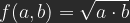
Multiply

Multiplication is one of the simplest blends, because the function does not give any values outside the allowed interval or 0 to 1. By the way, PS indeed uses multiplication, not the geometric mean, though the latter might seem more plausible.

$f(a,b) = a \cdot b$

Results for a and b between 0 and 1 lie within that interval as well.

For my test images you get:

$f(x,y) = a(x,y) \cdot b(x,y) = x \cdot y$

Looking at the result you can see that two edges and hence three of the corners should be black, because a multiplication with 0 always yields 0. Only in the top right corner you get a value of 1 for white.

Multipy

Aside: Geometric Mean (not available in Photoshop)

For me the geometric mean

$f(a,b) = \sqrt{a \cdot b}$

seems to be the better option. There’d be a nice linear transition along the diagonal.

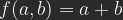
Linear Dodge

Linear Dodge is the name given to the addition. It is immediately clear that an addition of two numbers between 0 and 1 yealds results between 0 and 2. For half of the pixels the results get truncated to 1. Used on photos, this can easily lead to burnt out areas.

$f(a,b) = a + b$

If the sum a+b gets larger then 1, it is replaced by 1. The formula never gives results below 0 anyway, so no truncating there. Hence you’d expect white on and above the diagonal between top left and bottom right, below that a linear gradient down to black in the bottom left corner.

Linear Dodge

Linear Burn

This is the negative inverse of linear dodge. It is the same as problematic on photos, you might get fully black areas.

$f(a,b) = a + b - 1$

If the sum a+b gets less then 1, f is replaced by 0. Values above 1 are never reached anyway, no truncating. Hence you’d expect black on and below the diagonal between top left and bottom right, above that a linear gradient up to white in the top right corner.

Linear Burn

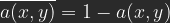
Linear Light

Frequently you will find linear light described as a combination of linear dodge for $b<0.5$ and linear burn for $b \geq 0.5$ . Not quite right, but close. If for $b \geq 0.5$ you compress the formula for linear dodge on the b-axis by a factor 2 and shift it up that axis by 1/2, and then also compress the one for linear burn for $b \geq 0.5$ by a factor 2 on the b-axis, you indeed get:

$f(a,b) = \left\{\begin{array}{lr} a+2b-1 & \text{for } b < {1/2}\\ a + 2(b -1/2) & \text{for } b \geq {1/2} \end{array} \right.$

Or, by resolving the terms, simply:

$f(a,b) = a + 2b - 1$

This is no longer commutative in a and b. Swapping the images A and B will yield a different resulting C.

Along the left edge (a=0) you expect black from the bottom up to b=0.5, then a linear transition to white. On the bottom edge (b=0) just black, because the -1 makes sure all possible results are negative. For b= 1 you get white on the top edge. On the right edge (a=1) you get from b=0 to b=0.5 a linear transition from black to white, above that just white.

Lineares Licht

Of interest for the PS user is the fact that an image B with $b=0.5$ for all pixels transfers image A unchanged to C when combined with this blend mode. $b=0.5$ is 50 % grey, which is called the neutral colour for linear light. Linear light is often used to manipulate a photo by using an almost grey layer with only minimal deviations, for example in high-pass sharpening or as one step of the frequency separation method.

Linear light can be described as the sequential execution of linear dodge and linear burn (with B multiplied by 2) or as linear burn with doubled B. The latter unfortunately cannot be recreated in PS, as it would need multiple steps, one of them yielding results outside the allowed interval. Intermediate results would be truncated, the main result would be wrong.

$f(a,b)= (a+b) + b - 1 = a + 2b - 1$

Other parts of this mini-series

Blend Modes – Part 2: Color Burn, Color Dodge, Screen, Overlay, Hard Light and Vivid Light

Blend Modes – Part 3: Soft Light

Sources
31. December 2014
Wie fotografiert man Träume?

Dritte Aufgabe des VHS Kurses: Wünsche und Träume. Wir sollen uns überlegen, was wir für Wünsche und Träume haben, und versuchen, diese in Bilder zu bringen. Der Kurs gewinnt langsam einen zu großen therapeutischen Anteil. Im letzten Monat war die Aufgabe, uns selbst zu fotografieren – ganz oder in Teilen, gespiegelt, als Schatten, wie auch immer. Schon das war eine ziemliche Herausforderung, bei der meine Kreativität ein wenig schwächelte. Und jetzt das. Habe ich noch Träume? Habe ich Wünsche, die ich positiv formulieren kann und die substanziell genug sind, sich in einem Foto darstellen zu lassen?

Ich fürchte, mein Selbstbild ist erschreckend und ich muss eine weiße Wand ablichten 🙁

23. April 2014